---

In the first article we explored the perceptron, which is a model that is able to classify a linearly separable set of inputs. Now you might have wondered, how does this help us do object recognition or build Chat-GPT? Well unfortunately we live in a world where not all problems are linearly separable, but are more complex. During the 1950s the excitement around the perceptron was short-lived, as the limitations were quickly realised. As famously pointed out in the book Perceptrons: An Introduction to Computational Geometry. It explained that the perceptron could not solve linearly inseparable problems such as the XOR gate problem. After this period the world entered what is more commonly known as the ‘AI Winter’, which was a period of time when it was difficult to find funding for any AI related projects, as overcoming the limitations of the perceptron proved to be a challenge. During this time it was however theorised that stitching together multiple perceptrons would overcome the limitations of a single perceptron. However, no one at the time was sure how you would train such a model, the problem being that there was uncertainty around how to adjust the weights of the model in a sensible way. We’ll explore what this means during this article, the solution unsurprisingly being a bit of imagination and some mathematics. The breakthrough was that we could treat neural networks as differentiable functions, which means we could analyse how the parameters of the neural network contributed to its output. This allowed the development of what is now the core step in training all modern-day neural networks: the backpropagation algorithm.

The Problem

Consider the XOR gate, famous for being the exact counter-example for highlighting the limitations of the humble perceptron. Why? Well let’s take a look at the inputs and outputs.

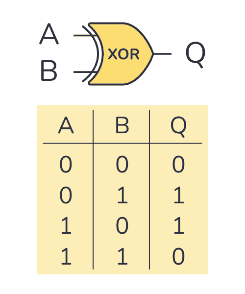
Conceptually an XOR gate is used to represent an exclusive or logic operation, which means it will only energize when one of the inputs is $1$, but not both. At a surface level it might not seem impossible for a perceptron to be able to predict the outputs of an XOR gate. If the perceptron was able to predict the outputs of an AND gate, what prevents it from predicting the output of an XOR gate? Let’s plot a possible decision boundary to see why this is not possible to do with a single perceptron.

From our plot we see that it is not really possible to divide the points using a single line, this tells us the problem is not linearly separable. Instead, we need a parabola to separate the points. In the context of AI non-linearity refers to anything that is not a line, so this parabola is a non-linear decision boundary. In the first article of this series, we learned that it is possible for perceptrons to discover linear decision boundaries, so learning the curved decision boundary for the XOR gate might seem like an impossible feat. Hope is not lost however, we just need to look at the problem from a different perspective, consider the following set of decision boundaries:

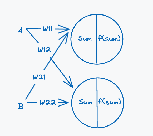
We see here that it is possible to separate the points using two lines, since we know a single perceptron can learn a single linear decision boundary the natural conclusion is that we can learn two decision boundaries using two perceptrons. That solves part of the problem, but it is not clear how these perceptrons would work together to solve the problem of predicting the output of the XOR gate. To analyse how to solve this problem we will look at a possible architecture for how we would train two perceptrons at the same time. Restructuring the architecture from the previous article to be able to learn two decision boundaries we get the following:

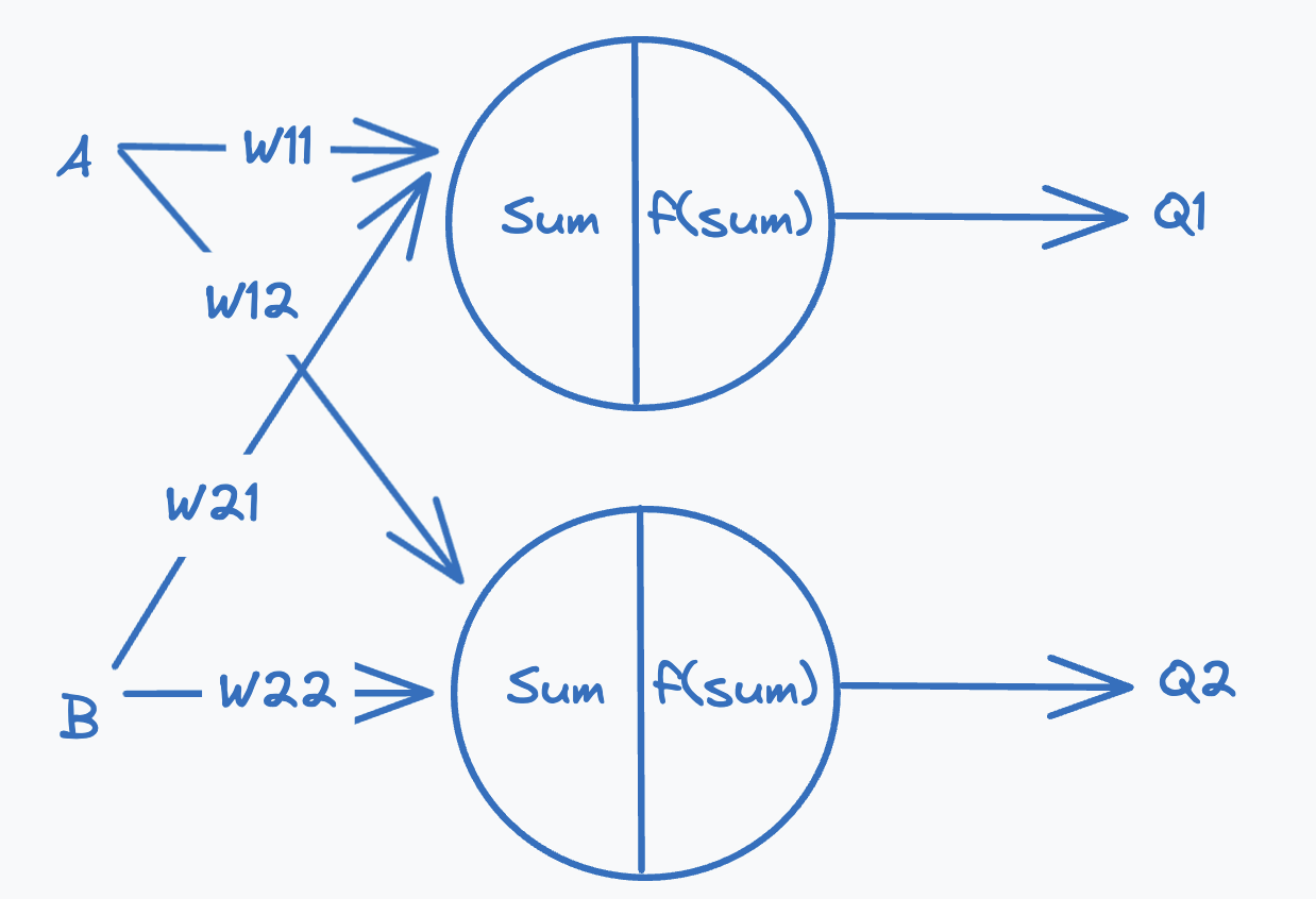
In the reworked architecture the input values A and B are passed simultaneously to both perceptrons, which perform two independent computations which will give us two outputs. Each perceptron has its own set of weights, which it will use as part of the computation. With this approach we have a way of generating two decision boundaries from the input data, but there is the issue that the perceptrons might end up learning the same decision boundary if the weights are initialised to the same value. We will not delve too much into this, so for now we’ll set it aside and assume the perceptrons will learn two distinct decision boundaries. To solve this problem we first need to define what the two decision boundaries would aim to classify.

A possible strategy here would be that each decision boundary should be able to learn when given the inputs $(0,0)$ and $(1,1)$ the output should be $0$. We know that the perceptron will only be able to classify whether an input is below or above the line. Considering the plot on the left-handside, it groups $\{(1,1), (0,1), (1,0)\}$ which we could train it to classify as $1$ and the input $(1,1)$ would falsely be correctly be predicted as $1$. This boundary does however classify the input $(0,0)$ correctly. The plot on the right groups the points $\{(0,0), (0,1), (1,0)\}$ together, but not $(1,1)$. Giving us a false positive for the input $(1,1)$. This is promising, the perceptrons should at least theoretically be able to classify three out of the four inputs, albeit for two different partitions of the input, but our two perceptrons will not be able to emulate the XOR gate with $100\%$ accuracy with these two decision boundaries. If the perceptrons work together they can make up for the mistake of the other perceptron. What if the outputs of the perceptrons were treated as the inputs for another third perceptron?

That could work, but before we construct an architecture for it, let’s analyse why this would work (theoretically). Fix the perceptron represented by the decision boundary on the left in Figure 5 to be perceptron $1$ and the right plot to be perceptron $2$. For this example, we make a bit of an obscure assumption, but will make sense in a second. Assume that the second perceptron will learn an inverse of the XOR inputs, this is so that the decision boundary will always output one for the partition of the inputs that contains $(1,0)$ and $(0,1)$. With this assumption in mind and using the decision boundaries as the indicators whether a perceptron outputs $0$ or $1$ we get the following table:

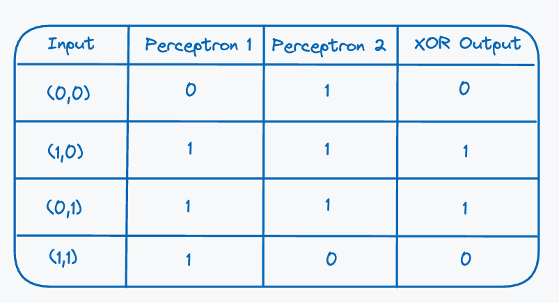
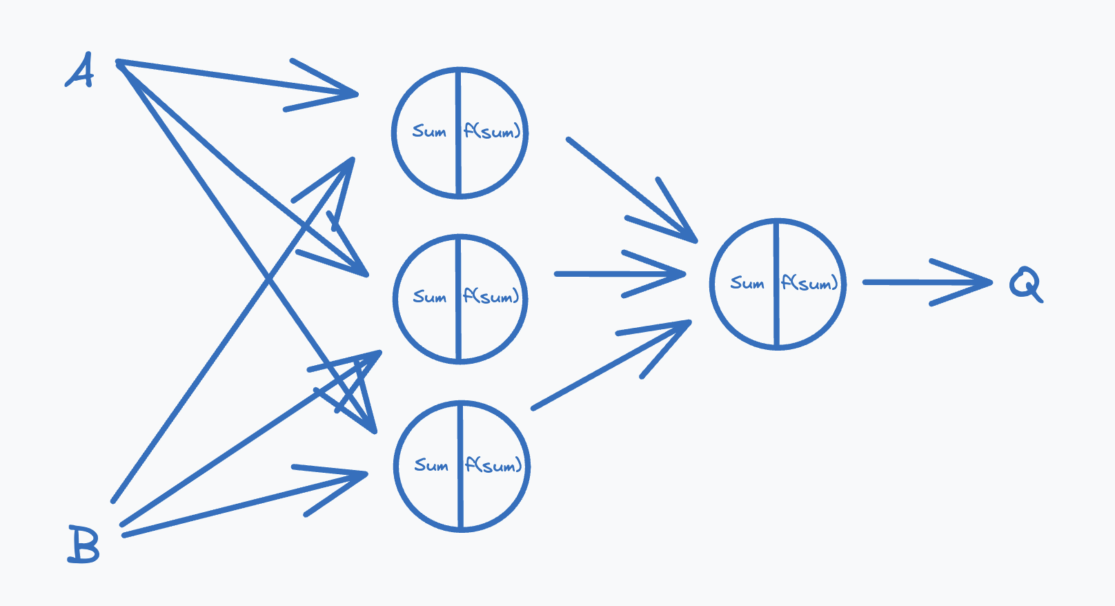
Here we see something interesting emerge, if we look at the outputs of the two perceptrons and the output of the XOR gate we actually see that it matches the inputs and outputs of an AND gate! We did make some assumptions, but we will see that this is actually close to what is happening. And as we saw in the previous article it is actually possible for a single perceptron to learn this successfully. We just need to feed the outputs of the two perceptrons into a third perceptron, which means we can then predict the output of an XOR gate. We call this third perceptron the output perceptron/neuron. So a possible architecture would look something like this(omitting bias for simplicity):

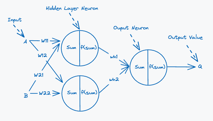
This architecture forms a neural network, a neural network is described in terms of layers. The inputs form the input layer, which is then fed into the hidden layer. Our hidden layer consists of two neurons and is responsible for preparing the data before sending it to the output layer. The output layer in our architecture consists of a single neuron and is responsible for producing the output value. The weights connecting the two hidden layer perceptrons to the output perceptron are labelled as $w_{h1}$ and $w_{h2}$. This all seems very promising and like theorised in the 1950s seemed to be a promising approach. However, this is all theoretical, and we have not trained the model just yet. Scientists discussed this as a possible model of how would solve the problem of predicting the output of an XOR gate and other more complex problems, but were quickly stumped when they attempted to define the training algorithm. The issue being that it was not clear how to update all the weights and biases in a meaningful way. How would you propogate the error value from the output perceptron to the previous two perceptrons that fed into it. Issue being that the perceptrons feeding their outputs into the last perceptron don’t know that they are actually predicting the output of an XOR gate, they just know they are feeding into some other output neuron. The output neuron is actually responsible for producing an output, which will in turn dictate the error value. This issue stumped AI researchers for quite a few years, this is until the discovery of the backpropogation was made.

Calculus To The Rescue

To train a neural network successfuly for a particular task you need to mimise some predefined loss function, much like with the perceptron. On that point let’s take a step back and take a look again at how training a single perceptron works, by looking at how it learns the optimal decision boundary. Learning the decision boundary is simply a side effect of minimising the loss function. Consider a simplified perceptron which only takes a single input value, the computation it performs given an input value $x$ is expressed as: $x \times w + b$ (ignoring the activation function for now). Experiment with the sliders to see if you can get the loss to reach $0$.

In the exercise above you probably used the line as an indicator, which makes the problem pretty simple. For a second challenge try and only use the loss value as the guide and see what you can achieve. This should a bit more challenging, but not impossible. The strategy to solving this problem (not looking at the target line) would be to keep an eye on the loss value. If the loss increases based on the weight or bias change the logical step would be to move it in the opposite direction. After some tweaking you should be able to achieve a loss value of $0$. What this exercise shows us is that perceptrons are trained by adjusting some set of parameters with respect to the loss value. Also, you might have also realised that as the error became smaller you also would’ve made smaller updates to the weight and biases. This fact also shows us that the magnitude by which the parameters are updated has a direct relationship with the magnitude of the error.

In the first article I mentioned that a perceptron is a simply a linear function approximator, so this means that the perceptron itself is a mathematical function. Let $f(x, w, b)$ represent a perceptron which can be thought of as a mathematical function which takes three inputs:

• $x$: Input value(s) of the perceptron
• $w$: Weight value(s)
• $b$: Bias value

The function will also apply the activation function $\sigma$, which gives us the following definition for the function:

For simplicity the perceptron takes a single input value $x$, which means it also only has single weight $w$. This perceptron consequently only has two parameters that can be adjusted by the learning algorithm (one weight and one bias). Put differently it means that only two values affect the loss value. Let’s take a look at how we performed this parameter update in the perceptron learning algorithm:

This works since in the perceptron model every parameter has a direct impact on the output of the perceptron. What I mean with direct is that there is no layer between the parameters in the computation of the final output value. A layer might be another mathematical function. Recall that the computation a perceptron performs is described as $\sigma(w \times x + b)$, the weight and bias parameters are what the output is derived from. This is the core issue with adding layers of perceptrons, what would it mean to change the weights in previous layers, that were not directly involved in the output calculation, but rather indirectly.

Looking back on the layered approach we took in constructing the neural network in the previous section, if we could establish a relationship between the parameters of the perceptrons and the final output of the neural network, we could then determine how the weights and biases should be updated. Expressed differently we want to know how to change the weights and biases with respect to the error/loss value. To be able to do this we need to change our views of a neural network slightly. We’ve been hinting at this fact, perceptrons can be seen as mathematical functions so a multi-layer network could then also be expressed as a single function composed of sub-functions. Taking our theoretical XOR gate neural network architecture we could rewrite the computation it performs as:

where

where the outputs of the perceptrons in the first layer are represented by $g(x, w, b)$ and $k(x, w, b)$. Let the error value be the mean-squared error expressed by the equation:

where $n$ is the number of possible input pairs (four in this case), $\hat Y$ is the actual output of the XOR gate. Notice that the loss function $\mathcal{L}(\hat y, f(x, w, b))$ is composed of the output of neural network $f(x, w, b)$, much like how the output is composed of $g(x, w, b)$ and $h(x, w, b)$. Now how do we define the relationship between the output $f(x, w, b)$ and the loss value $\mathcal{L}(\hat y, f(x, w, b))$? Well we need to reach for some calculus. Calculus is the study of continuous change, it is a branch of mathematics that uses constructs to reason about change and rates of change. We want to know how we should change the parameters of the neural network to minimise the error/loss value.

The construct from calculus that we will use to inform the parameter adjustments of the neural network is known as a derivative. A derivative describes the rate of change of the output of a function with respect to a certain variable. So in our scenario we want to quantify the rate of change of the error with respect to a neural network parameter. To express the change in the error with respect to a single weight we express it as:

The expression above is not entirely accurate, it is only used as surface-level introduction to the syntax of calculus. There are two things wrong, the first thing being that since the loss function is a multi-variate function, which means it takes more than one variable as input. Our loss function takes the actual output of the XOR gate $\hat Y$ and the output of the neural network $f(x, w, b)$. We only care about the change of the output our neural network, so we want to calculate the partial derivative of the loss function. Furthermore, the network output is also parameterised by other functions and variables (its own weights and biases). So the correct notation to express the change in the error with respect to single weight in a multi-variate function would be:

This derivative quantifies the change in the error with respect to some weight parameter $w_{ij}$ in our neural network. One thing I’ve failed to mention is why this rate of change is useful in informing the network parameter adjustments, to better explain this we look at the concept of a gradient. To understand what a gradient is, let’s quickly gain an intuition for what a derivative actually is. Practically the derivative is described as the instantaneous rate of change at a point. Consider the following visualisation (move cursor along curve):

The derivative $\frac{dy}{dx}$ of the above parabola $y = x^2$ is a line. The slope of the line describes the value of the derivative at that point. The point at which the derivative $\frac{dy}{dx} = 0$ is when there is no change or the slope of the tangent line is $0$. To understand why this is useful, imagine this parabola represents all the possible loss values for a perceptron with a single weight and no bias. This means the value of x-axis is the value of the weight and the y-axis is the value of the loss. Since we want to minimise this error value, it would be useful to know at which point the loss value is $0$. The derivative is a useful tool in determining this point. So the problem of minimising the loss value can also be thought of as minimising the derivative value of the loss function with respect to a parameter of a perceptron or neural network. Now this only looks at a single parameter, if we add another parameter we end up with a loss landscape as shown in the first article. However we mentioned that a derivative represents the rate of change for a single variable, so how does the calculation work for multiple parameters? Well the partial derivative partially :) solves the issue. Consider some generic loss function $\gamma$ for a neural network with $m$ weights and some number of biases. For the sake of argument we’ll only be looking at the weights, but the principle is the same for the biases. Calculating the partial derivatives for the loss function $\gamma$ with regard to the weights would result in the following:

This list of partial derivatives actually defines the gradient of the loss function $\gamma$. Like the derivative the gradient represents the slope of $\gamma$, i.e. the gradient points in the direction of the greatest rate of increase in the function. To visualise this fact consider a simple example loss landscape for a single perceptron with two weight values:

For this bowl-like loss function its gradient would be given by:

The gradient is more formally expressed as:

Now to visualise the value of the gradient $\nabla \gamma$, we can derive a contour plot from the loss landscape. Imagine the contour plot as squashing the loss landscape to 2 dimensional plane. The gradient can be visualised as an arrow that will always reliably point in the direction of the greatest increase. In the plot below the darker the values get the lower the value of the loss function. If you hover on any point on the plot you will see that the gradient will always point in the direction of the steepest increase.

By simply negating the value of the gradient we can get the gradient to point in the direction of the steepest descent.

So with this useful construct in hand let’s revist the problem of optimising a neural network. The goal with training a neural network is to instill knowledge. The parameters of the neural network are responsible for capturing and holding the knowledge of the neural network. One of the ways of training the network is learning by example. Given some piece of data a neural network should be able to reason about it and report some conclusion to its reasoning in the form of an output. The network learns when we tell it how far it is from the expected output, the distance between its answer and the expected output is the error. The error is a point on the loss landscape for the chosen function used to calculate it. The loss function is (logically) parameterised over all the variables of the neural network so it is possible to reason about the change in the error with respect to each parameter that contributes in the loss function and hence the error/loss value. The partial derivative captures the change in that error value with respect to a single parameter. This allows us to answer the question to whether a specific parameter increased or decreased the error value. So this means instead of adjusting a weight or bias using the error value as we did in the perceptron learning algorithm, we use the partial derivative instead. Since the partial derivative becomes our new error value, we still make use of a learning rate to scale down the derivative value. So the step for updating the weights and biases for a single perceptron would be given by the following:

Something I’ve not mentioned is that the expression $\frac{\partial \gamma}{\partial w_i}$, is actually a bit more complex. Let’s use a more concrete example, looking at the mean-squared error function to elucidate this a bit more:

To calculate the partial derivative of the mean-squared function, you only look at squared part of the expression. I will not be going into the specifics to why you do this and go into the specific of how to derive the partial derivative, as this is not the goal of this series and is not critical to gaining an intuition for what is happening.

The partial derivative of this expression is expressed as:

Since the loss function is composed of a second function $f(x,w,b)$, the output of the neural network, the partial derivative of that function also needs to be calculated. In the world of calculus this rule is aptly named the chain rule. This rule is useful since the loss function itself is not directly parameterised by the weights and biases in the output and hidden layers. So the expression for deriving the change in the MSE loss value with regard to a weight $w_{hi}$ in hidden layer of the neural network:

The weights connecting the inputs to the two hidden layer neurons the expression is slightly different, consider for a weight connecting the neuron given by function $g(x, w, b)$:

For the sake of clarity the change in loss w.r.t to the weight connecting to the neuron given by $g(x, w, b)$:

Now after a lot of scary notation we have finally solved the problem of how to relate each and every neural network parameter to the loss function, furthermore we can also derive whether to increase and decrease those parameters based on a loss value. With this we can once finally describe the learning algorithm for a multi-layer perceptron network.

Transformations

The algorithm for training is pretty similar to the perceptron learning algorithm, just with a different optimisation step. Before we look at the training algorithm, let’s take a more in depth look at how a neural network transforms data. Recall that the computation a perceptron performs is given by $\sigma(wx + b)$, where $w$ is a vector connects each input to the perceptron. With this computation it was relatively simple to think about how the perceptron was transforming the input, in essence it was simply scaling the inputs. We’ve been able to reason about the transformation a single perceptron performs, but now we need to reason about how a layer transforms the inputs or the outputs from the previous layer. Before we look at the transformation, we need to first understand what a matrix is and the role it plays in a neural network. To explain what it is, we’ll look at how we can compute simultaneously calculate the output of the perceptrons in the first layer of the XOR gate neural network:

First we need to calculate the weighted sum for each perceptron, for this let the input be a vector consisting of input A and input B: $\langle A, B \rangle$. The weights we arrange in a grid, this is also called a matrix:

Calculating the weighted sum for each perceptron can be done by performing a vector-matrix multiplication:

The specifics of the multiplication steps are not too important, all we need to understand is it can be used to compute the weighted sum for both perceptrons at once. The cool thing is that this method scales to any number of neurons. The resulting answer is a vector for the weighted sum for each perceptron, this vector is then added to a vector of biases. The activation function is then applied to each element in the vector:

Now it can actually be a bit unclear as to what is actually happening here, so let’s see how we can visualise it. Using the problem of predicting the output of the XOR gate, the problem originally was that we could not create a linear decision boundary to separate the inputs of the XOR gate. We saw that we needed a more complex non-linear decision boundary or as we hypothesised using multiple decision boundaries to separate the data. This hypothesis is not incorrect, but I would like to show what the perceptrons are doing when looking at how they work together. The key to visualising this, is vector-matrix multiplication. Recall that a vector can be seen as an arrow that points to some point in a cartesian plane and goes through the origin of that plane. A matrix is some collection of points, but can actually be thought of as a function which can move the vector it is multiplied with. For simplicity assume we want to do the following multiplication:

For the visualisation let every point represent a vector or more specifically the end of a vector (the point it points to). Click transform to see how the matrix moves the different vectors (play around with different matrix values to see some other cool transformations).

The transformation the matrix applies is formally known as a linear transformation. The above example shows a rotation transformation, the main takeaway here is that the vector-matrix can move vectors around in some abstract space. The next step after multiplying the vector with the matrix representing the neural network weights is adding the bias vector. Recall that a bias is able to change the intercept point for the decision boundary for a single perceptron, it has a similar effect here where it will simply translate the vectors in either the $x$ and $y$ dimension (in this 2D example).

The next operation is applying the activation function to each weighted sum in the resulting vector after multiplying the input vector with the weight matrix and adding the bias. So now we quickly also need to address why our step-function from the last article can not be used in a neural network. The reason is due to the nature of derivatives can only be applied to continuous function. Recall that the step-function is $0$ for any value less than $0$ and $1$ for any positive number.

At $0$ the ‘instantenous’ jump happens where $1$ is returned by the function, the derivative of the step-function does not exist at this point and so we can not adjust the weights when the weighted sum is $0$. There is some more complicated mathematical logic behind this fact, but for the sake of argument just know that we can not use this function when using the backpropogation algorithm for updating the parameters of a neural network. So instead we will be looking at a new activation function more formally known as a sigmoid function:

The sigmoid is a smoothed out step-function and is trivially differentiable since it is continuous over all inputs. We can visualise the magnitude of the derivative for the different inputs of the function using the visualisation below:

With this last puzzle piece we can fully visualise how the first layer of the neural network manipulates the inputs given to it:

In the above animation you can see how the translations are applied in a step-wise function. The usefulness of these transformations might not be immediately apparent, but let’s think about this for a second. Remember that the output node of the neural network we built is only a single perceptron, which means it can only learn a single linear decision boundary. This means we need to find a way of transforming the inputs in such a way that the last output neuron can linearly separate the inputs fed into it. Preparing the input space is the responsibility of the hidden layer of the neural network. Let’s see if we can find the weight values and bias values by hand for the hidden layer (as a hint I’ve already set a possible set of weights, play around with the bias values):

After playing with the bias values you should see that if the bias vector is $\langle 1.5, -2 \rangle$, we are actually able to linearly separate the points that output $1$ from those that output $0$. This means that the perceptron in the output layer learns how to separate the points after they have been transformed. Once again we have analysed that our perceptron has an appropriate architecture and can learn the XOR gate. So for completeness let’s define the algorithm for training this neural network.

Training

Finally we have everything we need to start training and analysing a neural network. Before training let’s look at the algorithm:

1. Initialize the weights randomly in some range
2. Iterate over each row in the possible inputs from the XOR gate(Figure ...)
3. Calculate the output given the input
    3.1 Hidden Layer Output = Hidden Activation Function((A,B) * (Hidden Weight Matrix) + b)
    3.2 Output = Output Activation Function(Hidden Layer Output * (Output Weight Matrix) + b)
4. Calculate ∂Loss / ∂(w/b) for every weight and bias in the neural network
5. Update every weight and bias:
    5.1 w' = w - learning_rate * ∂Loss / ∂w 
    5.2 b' = b - learning_rate * ∂Loss / ∂b
6. Repeat steps 2-5 a specified number of times

The process of calculating the output and the loss values is known as forward propagation (steps 2-3). Updating the weights and biases is known as back propagation (steps 4-5). These two procedures summarise the two phases of training a neural network. Below we show the loss graph for one of the runs of training a neural network. It was trained over $40,000$ epochs and a learning rate of $0.1$.

We don’t get a final loss value of exactly $0$, but would probably be possible if it is trained for longer. This is plot is interesting to look at, but to get better idea of how the network learned, we can actually take a look at the loss landscape.

Looking at this loss landscape we can see why the network took so long to train, it seems that the optimal loss value (purple) lies in a narrow cavern. Making it pretty difficult to find, but due to the smooth landscape the gradients would still be easy to follow. The landscape is however much more complex compared to the loss landscape in the first article. Before we move on let’s take a look at how the landscape changes when we change the parameters with which we trained the network. Instead of using the sigmoid activation function let’s see what happens when we use the hyperbolic tangent function. The hyperbolic tangent function ($tanh$) is similar to the sigmoid by squashes values in the range $(-1,1)$:

The landscape is a bit more shallow, which is more advantageous when training due to the fact that the gradients change more smoothly. This landscape is easier to train the neural network on since the landscape is smoother than the sigmoid landscape, the drops are a bit more gradual and don’t form extremely deep valleys. This means there are less abrupt steps that could overshoot good solutions. Numerically the hyperbolic tangent is superior to the sigmoid function due to its higher derivative values, meaning we can extract more information from the gradients. Higher error values makes the backpropagation step more meaningful. Consider the plot below comparing the sigmoid and hyperbolic tangent derivative values (click on legend to hide certain plots):

In the above plot we see that the $tanh$ function has a steeper increase around $0$ when compared to the sigmoid function. Is the hyperbolic tangent function the best we can do? No, we can actually do better, let’s consider a bit of an obscure function called Mish. The Mish function is plotted as follows:

The function is a weird one, the reasoning behind the function is that it will ensure large activation values when the input is positive and will fix anything that is negative to be close to $0$. It allows smaller activations when the input is around $0$, to allow for non-zero gradients which still allows gradient information to flow through the network when the activations are small. The reasoning for linearly scaling the positive inputs is to allow for sparse activations between neurons, meaning that neurons do not fire at the same time. This is not too important in our toy neural network, but is still good to know. Let’s compare it with the sigmoid and hyperbolic tangent functions to analyse its usefulness:

Comparing the derivative values, we see that as the input gets larger the derivative will get closer to $1$, whereas the sigmoid and $tanh$ derivatives get closer to $0$. Also for negative values it still ensures that the gradient value is close to $0$, but not exactly so it still allows gradient information to flow back through the network. Let’s discover how the Mish function affects the loss landscape for our neural network:

The Mish function gives us the best possible loss landscape. This is due to the optimal loss value region is flat and much larger than $tanh$ function and sigmoid functions. This means it is simple for the neural network to learn. The landscape even though flat is smooth, with no local minima so following the gradients will take you to the most optimal loss region. To reinforce the impact the Mish activation has on the training a neural network, we can plot the loss values of the epochs during training:

The neural network as able to learn the XOR gate output in roughly $400$ epochs, which is a huge improvement to the sigmoid activation function.

A More Complex Problem

To further solidify our understanding of neural networks, we need to be able to answer two questions ‘what happens when we add more neurons?’ and ‘what happens when we add more layers?’.

To answer the question of adding more neurons we’ll use an example dataset which requires at least three neurons in the hidden layer:

This two circles dataset is a classic example in showing the importance of dimensionality in a neural network. This particular dataset can not be learned by our current XOR gate neural network architecture. The reason being that the dataset can not be trivially transformed in such a way that the points can be linearly separated in two dimensions, but it is possible to do by adding another dimension. We’ve only looked at decision boundaries in a 2D space, but if we add another neuron to our hidden layer we can project our 2D input ($x$ and $y$ values of points) into a 3D space. So let’s ammend our XOR gate neural network architecture to the following:

By adding the third neuron in the hidden layer, we can project the two dimensional to a three dimensional space. Training a neural network on this dataset for $2,000$ epochs and a learning rate of $0.01$ we get the following transformation in the hidden layer:

Rotating the plot a bit you should see how the points could be separated by a hyperplane. You can imagine a hyperplane as a piece of paper that you can use to separate data points.

Now that we know that adding neurons to a layer increases the dimensions into which the input space is projected, what happens when we add more hidden layers to our neural network? Recall that every layer performs a transformation on the inputs from the previous layer which might be the input or the output of another perceptron. With the addition of the activation function we can get some complex transformations that we might not have been able to see as a possibility. The result of every transformation is commonly referred to as a representation, a neural network when trained as we saw will try to find a suitable representation for the data such that it can more easily classify the data. Adding layers to a neural network result allows it to learn more complex patterns. It is easier to solidify this idea when talking about deep learning models such as CNNs and even transformer models, which will look at in the next article. For now, you can imagine that by adding another layer you are adding another type of transformation that is able to fold, rotate and scale the outputs from the previous layer. If the layer has more neurons than the previous one it is also able to create a representation in a higher dimension which might be able to better separate the data.

Conclusion

Phew! That was a lot of information, but we now have working knowledge about how neural networks work, we understand how they manipulate data, we have a functional understanding of how they can be optimised for the task we want them to perform and finally we have a basic understanding of what happens when extend the depth and width of the neural network. The next part in this series will start exploring the concept of deep-learning, we will look at problems requiring 10s or 100s of neural network layers to be able to understand them fully.

Further Reading / Blog Inspiration

• Visual Explaination of Linear Algebra and Linear Transformations
• Useful Explainer For Understanding Backpropagation
• Cool Loss Landscapes For More Complex Neural Networks
• Topological Approach To Understanding Neural Network Transformations(Written By Anthropic AI Co-Founder)
• Awesome Research On Topological Properties of Neural Network Transformations
• THE Research Paper On Visualising Neural Network Loss Landscapes