---

The year is 2024 and there are walking-talking robots, we are catching rockets and have driverless cars. I want us for a moment, to take a step back in time, to the year of 1940 in the city of Bristol. Here we will find a neurologist by the name of Dr. William Grey Walter who unknowingly designed one of the earliest forms of what would later be referred to as Artificial Intelligence. His battery-powered robots were models to test his theory that a minimum number of brain cells can control complex behavior and choice. A rotating photoelectric cell, the machine’s “eye,” scans the horizon continuously until it detects an external light. Scanning stops and the machine either moves toward the light source or, if the source is too bright, moves away. He claimed that these robots had the equivalent of two whole neurons and further speculated that by adding more neurons they would only become more intelligent (spoiler: he was right).

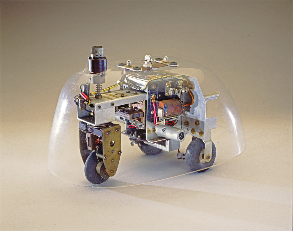
Now this robot marks the first example of AI and robotics, but this is not the first occurrence of ‘computer learning’ as the robot was purely mechanical, but still captured one of the core tenets of Artificial Intelligence: “cognition is recognition”. This statement describes that the process of acquiring knowledge and understanding is through the identification of something from a previous encounter. The argument aligns with how we as humans learn and reason, if we see a dog, we only recognise it as a dog because we were told it was a dog in a past encounter. Even though this alignment exists we are still unable to fully reason about how AI systems are able to learn and why they work. However, this does not mean we can not discover insights into how they work. Now there are two avenues to understanding AI systems, for the mathematical wizards among you, you might reach for a calculus and linear algebra handbook to gain that understanding, but I want to propose a second avenue, rather than focussing on the complex mathematics that make AI systems tick, we will attempt to build an understanding on top of visualisations from zooming into the internal components of modern day AI systems. This series will focus on taking an illustrative approach to explaining how different types of neural networks and their respective algorithms work. The series will take some ideas from an emerging field, mechanistic interpretability, which seeks to understand the internal reasoning processes of trained neural networks. It will aim to build this understanding by incrementally introducing the various building blocks of modern day neural networks.

The Perceptron

---

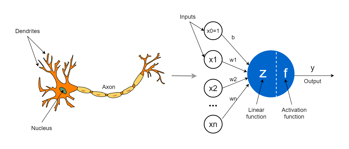
The ‘Tortoise’ robot was a mechanical robot and consequently did not follow a computer program, the concept of ‘computer learning’ would remain a mystery until the year of 1957. This is when Frank Rosenblatt developed the perceptron model, the first model that was able to successfully simulate the human cognitive process at a base level. His discovery is regarded by most as the match that started the wildfire, that is Artificial Intelligence, that has continued to spread to this day. The perceptron model is still used today to describe the most simple form of neural network. A perceptron (also called a neuron) is meant to represent a single biological neuron. In the perceptron model it takes one or more inputs or stimuli and will then decide whether to ‘activate’.

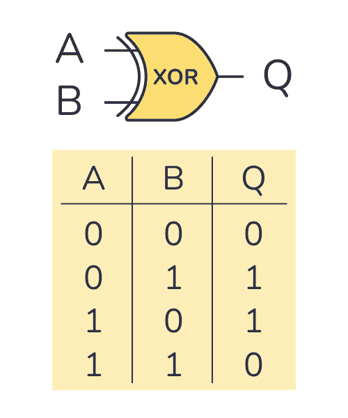
To get a better intuition for the perceptron model we will use an example scenario, consider the scenario where you want to predict the output of an AND gate. An AND gate is a digital circuit that is energized when, both of its inputs are energized. To model this conceptually we say that the circuit will return a value of 1 when both of its inputs are $1$ and $0$ otherwise. We summarise the behavior of the AND gate in the table below:

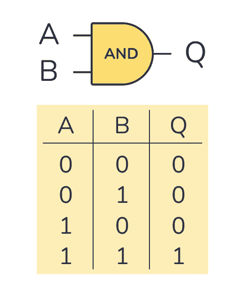
A and B are the inputs to the AND gate and Q is the variable representing the output of the AND gate. If we plot the possible inputs of the AND gate, we see something interesting emerge.

We can clearly separate the points using a single line, where the points below the line mean the AND gate will output $0$ and the point above the line will output $1$. This line is conventionally called a decision boundary. This phenomenon means that the problem of predicting the output of an AND gate is linearly separable. Meaning that we can separate the data into two classes using what is formally known as either a line or a hyperplane (for higher dimensions), put simply, it means we can construct a plane between the data points such that we can classify the points into two distinct classes. More specifically a perceptron with $p$ inputs is considered to be a linear function approximator and can be used to approximate any function of the form:

The problem of approximating $f(w)$ is reduced to estimating $\beta_0,\beta_1,...,\beta_p$ such that the output of $f(w)$ matches the desired output. In our scenario we only have two inputs so the function we are trying to resemble looks like:

In this trivial example we can easily find the line by hand, but for the sake of argument we will assume that we can not easily find this line (this is the case for more complex problems). As we will see later this equation is actually related to the standard form of a line($Ax + By = C$), which is why a line is used to separate the data. We will explore a bit later why the perceptron is suited to solve the linear separability problem.

A perceptron is a mathematical function which is given a list of input values, and it produces a single output. A perceptron computes the output by performing a weighted sum between the input values and a list of randomly initialised weights and feeds the result through an activation function to obtain an output. The activation function is responsible for determining whether the neuron should fire and is consequently usually a function that returns some value between $0$ and $1$. Relating this back to the identified core tenet, the activation function can be thought of as the decider whether it recognises a piece of input. Conceptually this means the AND gate will learn to only activate when $A = 1$ and $B = 1$ is presented to it. We will look at a special type of activation function that will always output either $0$ or $1$, since these are the only valid output values for an AND gate. Below we define the ‘architecture’ of the perceptron for predicting the output of an AND gate:

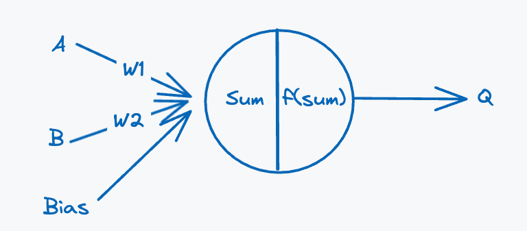
The perceptron has a special third input called the bias, we discuss the role of this component in the later sections. The weights describe the state of a perceptron, they encode what the perceptron knows about the input data. The weights encode this knowledge by describing how the perceptron should interpret the input data. They are responsible for preparing the data before passing it to the activation function, which will make the final decision whether the perceptron should activate or not.

Weights encode knowledge

Our perceptron takes two inputs labelled A and B (gate inputs) and a third bias input, the weighted sum is calculated by performing the following operation:

This is then passed through to the activation function, the activation function will return $1$ if the weighted sum is positive and $0$ if the weighted sum is less than $0$.

We choose the value of $0.0$ arbitrarily as it lies in the middle of $0$ and $1$, which is the domain of the input variables. This type of function is commonly referred to as a step function and is useful in our case for clamping the weighted sum to correspond to a valid AND gate output.

Training

---

Now how do we get the perceptron to actually emulate an AND gate? Well we need to train it. To train our perceptron to correctly predict the output of an AND gate, we need to train it on some examples. The possible inputs of the AND gate will be the examples which we will train our perceptron on(referred to as training data from here on). As said by author John Bradsaw “mistakes are our teachers”, the perceptron has no perception of what an AND gate is, so we need to instill this knowledge into the model using a trial-and-error algorithm.

Since we know what the output of an AND gate should be, we can label the inputs of the training data and ‘help’ the perceptron when it incorrectly predicts the output for a given set of data points. We do this by calculating the difference between the output of the perceptron and the actual expected output. This gives us an error, which we use to nudge the weights in a direction such that the output of the perceptron becomes closer to the expected output. The value of the error is what we want to minimise. To keep track of this error we will be using a more general loss function, the mean-squared error, this will allow us to reason about error values more easily. We will formalise the loss function as follows:

Now it would be useful if we could plot this loss function to get a better understanding of what our perceptron is trying to optimise. Using the weights and all possible real numbered values in the range $[-2,2]$ and the loss function definition we can calculate all possible error values for our input domain and plot them. Plotting all of these points allows us to construct what is known as a loss landscape.

A loss landscape is a visual representation of the ‘terrain’ our perceptron will have to traverse to find the weight values that minimise the loss/error value. The loss landscape is a valuable tool for gaining insight into model training dynamics. At a high-level we see a fairly flat landscape with a single funnel structure in the middle. The flat terrain can make it difficult for the model to learn, since changing the weights has no noticeable effect on the loss, so it is not clear which direction the minimum loss is. The flat areas of the landscape are commonly referred to as flat minima. The landscape also has high ridges, where there is a steep increase in loss, which make it difficult for the perceptron to move through. It is also extremely useful in seeing the existence of optimal solutions, which in this case is where the loss is $0$. So if the weights are initialised between $-2$ and $2$ we can see that there is only one region of the landscape where the loss value is $0$. This region is a globally optimal solution, since the loss value is the lowest any learning model can possibly achieve in this specific problem.

With this in mind it should be clear to see that the initial value of the weights will impact how easy the perceptron will be able to find the optimal weight pair that minimises the loss function. Consider our weight values are initialised such that the loss function output value is on the top yellow plane. We will have to traverse multiple flat minima until we reach the bottom of the ridges which will show improvement in the loss function value. The loss landscape has given us the ‘answer’ to our perceptron learning problem, but quickly becomes infeasible to construct for more complicated problems as the number of weights is typically in the millions, so is typically only used for visualisation of simpler AI models. This is however a nice guide, since we know what values we need to work towards for the weights of the perceptron. To train this perceptron we will define a simple algorithm:

1. Initialize the weights randomly in the range [-2,2]
2. Iterate over each row in the possible 
   inputs from AND gate table(Fig. 2)
3. Calculate the weighted sum: (A * w1) + (B * w2) + b
4. Apply activation function 
5. Calculate difference between value from activation function 
   and the actual expected AND gate output value: L = expected - predicted
6. Update weights according to difference: 
    6.1 w1' = w1 + learning_rate * error * A
    6.2 w2' = w2 + learning_rate * error * B
    6.3 b'  = b  + learning_rate * error
7. Repeat 2-6 some amount of times until satisfactory

The perceptron learns by repeatedly trying to predict the AND gate output given an input sample. It computes this output by performing a weighted sum. To better explicate what this weighted sum is doing we rewrite the formula using an operation from linear algebra:

The weighted sum is done by performing a dot product over the vector of the inputs ($\langle A, B \rangle$) and the vector of the weights ($\langle w_1, w_2 \rangle$). A vector can be thought of as a list of numbers, which can be interpreted geometrically as an arrow that goes through the origin of a Cartesian plane and ends at the point given by all the numbers in the vector. A coordinate on a xy-plane is referred to as a 2-dimensional vector. Vectors can be n-dimensional, so the dimensionality of a vector depends on the number of values it contains. Consider two vectors $\langle 1, 2, 3 \rangle$ and $\langle 4, 5, 6 \rangle$, the dot product can be visualised geometrically as follows:

A dot product between two vectors can be interpreted as a measure for how much of one vector lies in the direction of the other. The green line gives us an indication of this projection, but is not the actual answer to the dot product and is only used as a visual aid. Fundamentally the dot product measures how much two vectors point in the same direction, so calculating this between the input and weight vectors tell us how many inputs relate to the weights of the perceptron. Put differently it tells us how much the input data aligns with what the perceptron knows, since the weights encode the state of the knowledge of the perceptron. The closer the input data is to what the perceptron knows the greater the chance for activation. So when we give the perceptron a specific input all it is doing is translating those points using a simple projection. This is another important insight into how perceptrons work and will become more clear when visualising more complex neural networks consisting of multiple of perceptrons.

Perceptrons perform geometric transformations

By updating the weights we are indirectly traversing the loss landscape, since the loss value dictates the direction in which the weights are updated. You might have noticed a new variable learning_rate, the learning rate is usually a value between $0$ and $1$ and is used to scale down the magnitude of the error value. The input values are included in the weight update to also help in scaling the weight value to be closer to the input, so that the magnitudes of the weights still make sense.

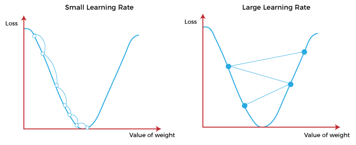
To better understand the optimization step (6) in Algorithm 1, consider a sticky ball that we place on some random point on the loss landscape with a position corresponding to the values of the weights ($w_1$ and $w_2$), where the position of the ball maps to the corresponding loss value of the perceptron. Since the ball is sticky and therefore also not affected by the slope of the landscape, it needs to be rolled to move. The direction we roll the ball in depends on the error and the amount of force we apply depends on the learning rate and the error. A higher learning rate can be detrimental when training a perceptron or a neural network since if you apply a lot of force the ball might overshoot its target (Figure 5: Right). So generally learning rates are set to very small numbers, but this is still problem dependent and can be experimented with.

With this background, we can now look at an execution of our learning algorithm. The parameters will be set as follows:

Here we see that our perceptron was able to successfully learn to emulate the AND gate after roughly $20$ iterations(epochs). Plotting the loss values over the epochs we can relate the loss values to the loss landscape from Figure 7. For the first few iterations we see that the perceptron gets stuck in the flat minima regions of the loss landscape, and it also struggles with the ridges as it oscillates between $0.25$ and $0.5$, but luckily it seems to find a path from the flat minima to the global optimal solution. To better understand these loss values let’s take a look at the values of the weights during the training process to see if we can plot the path through the loss landscape:

The final weights obtained are $w_1 = 0.15$ and $w_2 = 0.5$. The final bias value was $-0.6$. The weights seemed to move closer to each other over the epochs. This emerging behavior shows us that the model seemed to scale the value for input $A$ higher than input $B$, but this is due to the initial weights. If the weight values were reversed the opposite would be true. To better understand why these weight values make sense, let’s try to predict the output given $A$ and $B$:

Here we see that the perceptron purposefully set the bias to be slightly less than the summation of the weights when both inputs are $1$, which gives us a value greater than $0$ causing the perceptron to fire. This means that if any of the inputs are zero, the weighted will be less than $0$, so the activation function will return $0$.

With these final weight values and past weights we can also plot a path through the loss landscape. Sampling the weight values from the loss function every four epochs, we get the following trace:

We clearly see that the perceptron was somehow able to even through the flat landscape ‘know’ where an optimal solution lied. I unfortunately believe this to simply be a coincidence as the optimal solution required the weights to be positive and close to $0$ and during the training algorithm the weights were both lessened each epoch.

Turning our attention back to Figure 4, we look at the decision boundary the perceptron found. The decision boundary is a straight line, we need to find the equation of the line to draw it. Looking at the weighted sum again we see something interesting:

This aligns with the standard form of a line:

Rewriting using perceptron variables:

We can rewrite this in the more common slope-intercept($y = mx + c$) to make it easier to plot, by keeping $w_2$ on the right-hand side:

With the slope-intercept equation in hand we can now substitute the variables we obtained after training the perceptron:

Finally, we can plot the decision boundary:

The perceptron actually found a very similar decision boundary to the one we drew by hand in Figure 4. This visualisation also presents the role of the bias input, a seemingly worthless input value, but is actually used to move the decision boundary. Without the bias input the decision boundary line can only go through the origin as the line intercept would be $0$. We can also see the evolution of this decision boundary during the training process:

This shows us how the perceptron was able to approximate the linear function $f(w)$ representing our AND gate. Now this one example solution found by the perceptron, as we saw in the loss landscape in Figure 7, there are a few other possible global optimal solutions, so I encourage you to play with the perceptron parameters in the training script.

What’s Next?

---

Our perceptron was able to easily learn to emulate an AND gate, but what about an XOR gate? An XOR gate or exclusive or gate, is a circuit that is energized when exactly only one of its inputs are energized.

Plotting the possible input values and their corresponding activations, we get the following:

Here we see that we can not separate the points with a straight line, but rather with a non-linear hyperplane. We can also only do this separation it seems like we need to do this in a third dimension. To find this hyperplane we will need a more complex transformation, as we can not linearly separate the points. This means we can not linearly transform the input data using a single perceptron, but maybe if we could combine multiple perceptrons we might be able to do a more complex transformation. Stay tuned for Part II…