---

Wait, Part 2 and a ½? Let me explain. While I promised that the next part of this series would dive deep into the coolest aspects of Deep Learning, I realised there’s something essential we should explore first—a quick but fascinating detour. Think of this as the appetiser before the main course. In the last post, we began demystifying neural networks, showing how they’re not just “black boxes” but powerful tools that transform and disentangle inputs to make sense of them. Now, before diving into the complexities of Deep Learning, I want to introduce you to something foundational yet extraordinary: embedding models. Embedding models are like translators for data. They take messy, high-dimensional information—like words, images, or even user behavior—and convert it into compact, meaningful representations that a neural network can easily work with. Imagine turning the chaotic world of language into points on a map, where similar words cluster together based on their meanings. That’s the magic of embeddings, and they’re the backbone of many modern AI applications, from search engines to recommendation systems. In this post, we’ll break down how embedding models work, why they’re so powerful, and what they reveal about the way AI understands the world. By the end, you’ll see neural networks in action in a whole new light. Let’s dive in!

Latent Spaces

There is a theorem called the Universal Approximation Theorem that is often quoted in the context of neural networks. The theorem gives us a guarantee that for a neural network with a hidden layer; given enough hidden units, it can approximate any function or put differently fit any dataset. The real intuition behind the theorem is not interesting because given enough hidden neurons you are just constructing a lookup table. So using a simple perceptron neural network, this means that for every possible input we could construct a neuron in the hidden layer that will fire for that particular input. However, this result is not particularly useful as having a neural network be a simple lookup table is not powerful. It also does not give an explanation for why neural networks are able to generalise and interpret data they’ve not seen before. The real reason seems to be in how they represent data.

As seen in the previous article, we saw that by using a trained weight matrix and multiplying it with the input vector, we can perform linear transformations on the input space, allowing us to unravel a new representation of the input space data points that was not apparent before. Recall the cocentric circle dataset:

Here the problem is to determine whether a point given by its $(x,y)$ coordinates belongs to either the inner or outer circle. We can formulate this as a binary classification problem, where we want the network to output $0$ when a point belongs to the inner circle and $1$ when it belongs to the outer circle. We saw that our network was able to transform these points such that it could separate the points using a single hyperplane (visualised as a flat piece of paper):

Now let’s reframe our definition and understanding of this transformed space. To explore this new definition let’s make use of an analogy. Neural networks interpret and reason about data much like how us humans process and engage with a book. For example, consider J.R.R. Tolkien’s The Hobbit. When reading the book, we don’t memorise every sentence word-for-word (unless you have a photographic memory). Instead, we construct an internal mental model of the story—key events, characters, relationships, and overarching themes. If someone asks, “How did Bilbo escape from Gollum in the cave?” we don’t need to refer back to the exact text to answer. Instead, we consult our mental model and recall that Bilbo used clever riddles to distract Gollum and eventually slipped away using the One Ring to become invisible. This internal representation enables us to answer questions without direct reference to the original source.

Similarly, neural networks don’t “memorise” their training data. Instead, they build internal representations or abstractions of the patterns within the data. These abstractions allow the network to generalise and respond to inputs it has never seen before. For example, a network trained to recognise handwriting doesn’t store images of every possible handwritten letter but instead learns features like curves, edges, and strokes that are characteristic of different letters.

In the context of neural networks, the space in which a neural network does its reasoning is sometimes referred to as the latent space. This space can be thought of as a transformed representation of the input space, in some cases it is also a compressed representation as it has lower dimensionality than the input space. Here the concept of a space is a bit abstract, imagine a space as a set or list of similar objects, an object could be anything, for example a number, words, image etc. A latent space has the property where similar items are positioned closer to one another. Similarity depends on the context of the dataset, in our cocentric circle dataset example distance is used as the measure of similarity. You could imagine your brain as a latent space or put differently: a compressed knowledge space of all your memories and experiences, the exact organisation of these neurons does however fall in the domain of neuroscience, so we use this idea as a loose analogy.

As mentioned in the first article the weights encode the learned features from the input dataset. The weights also play a role in parameterising the linear transformation of the input space, the transformed space becomes the latent space. The latent space is consequently structured by the weights, it should be clear that the latent space is thus a representation of the features. The latent space more specifically captures the underlying features of the data, which is not directly observable from the input data. Latent means hidden, so that is why we refer to this space as the latent space. We’ve actually seen an example of what a latent space might look like:

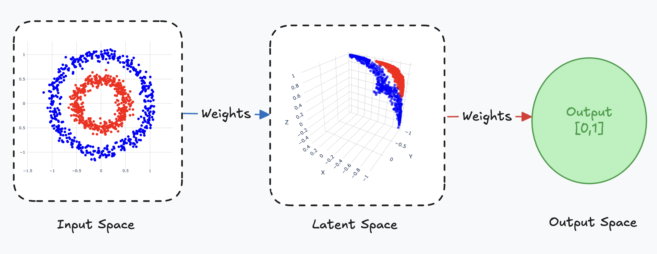
Here we see that the latent space still maintains the underlying structure of the input space, blue points are close to other blue points and the same for the red points. It also encodes a more abstract representation of the dataset, it disentangles the points to allow for separation.

Embeddings

Latent space embeddings, also known as embeddings, represent input data points in a continuous, possibly lower-dimensional space. While their significance might not be immediately obvious, latent spaces are remarkably powerful. They enable the computation of continuous representations for discrete data, and in certain applications, they allow for the generation of new data points due to the continuity of this space. In this article, we will explore the ability of latent spaces to create continuous representations, while their generative potential—such as in autoencoders—will be examined in a subsequent article.

To illustrate the power of embeddings, let’s consider how words can be embedded in a latent space to encode their meaning as vectors. This approach ensures that words with similar meanings are positioned closer to one another in the space. Word embeddings form the foundation of Large Language Models (LLMs), including the ChatGPT model suite. The intuition behind word embeddings can be traced back to John Rupert Firth’s 1957 statement: “You shall know a word by the company it keeps.” This idea suggests that the meaning of a word can be characterised by its surrounding context.

A word embedding can be thought of as a parameterised function, $\mathcal{W}$, which maps a word to a vector in the latent space. These vector representations capture the semantic relationships between words, enabling models to perform tasks such as language understanding, translation, and text generation with remarkable accuracy.

Where the vector is an embedding of the word in some high dimensional space, where the numeric data captures the contextual representation of the word. To actually visualise the usefulness of these embeddings you need to plot them, typically these embeddings might have hundreds of dimensions, so you need to apply a dimensionality reduction technique such t-SNE or UMAP. These techniques are incredibly powerful and complex, so they deserve their own articles. The exact inner workings of these algorithms are not too important to understand that they can take any $N$-dimensional vector and reduce its dimensions to a more visualisation friendly value such as $2$ or $3$. Consider the below visualisation of word embeddings generated by a trained embedding model:

Above you’ll see clusters of points, these are most useful for understanding the power of embeddings. If you hover over the points on the middle-left cluster, you’ll see that all the points are actually names, this is also true for the clusters close to it. For a nicer visualisation head on over to tensorflow projection it has a more interactive visualisation.

The embedding value is computed by an embedding model trained on some collection of text as the training dataset. What this means is we can establish semantic and syntactic word relationships. It has been discovered that with an appropriate embedding model we can use simple algebraic operations to reason about these semantic properies, consider the following:

This can be understood as removing the context where a “King” is a “Man”, but rather used in the context of a “Woman”. Now assuming you used an appropriate dataset and trained your embedding model correctly, the resulting vector would be close to the embedding for the word “Queen”. You might also be able to capture superlative forms of words, present participles or even country currencies:

Checking these relationships allow us to evaluate how well our model understood the semantic relationships between the words in the corpus. It is also important to note that these relationships do depend on the way they are used in the sentences that make up the chosen dataset, so as the model designer you need to be able to identify your own relationships in your chosen dataset to be able to evaluate the embedding model.

To be able to map a word to a vector, we need a lookup table where every word maps to exactly one embedding vector. We denote this matrix/lookup-table as $\theta$. Recall that a matrix is a grid of numbers described by some number of rows and columns. The number of rows in the matrix will be equal to the number of words that we are trying to embed, this collection of words is known as the vocabulary that we are trying to embed. The size of the vocabulary is determined by the number unique words in the dataset. The number of columns in the matrix is equal to the embedding length, which is the length of the vector we want to use to embed the words.

To get the embedding for a word we first need to convert it to a number which we can use to find its corresponding row in the matrix. This is done by building an index mapping a word to a position in the text it was extracted from. Take for example the following sentence:

The quick brown fox jumps over the lazy dog

The index would like the following:

So to retrieve the embedding for word “The”, we retrieve the first row in the matrix $\theta$.

The values in the matrix are extracted from the embedding layer from some trained embedding model. There are various techniques for computing vector embeddings of words that even extend beyond the world of AI, but in this article we will look at the Word2Vec approach.

Word2Vec

In the Word2Vec paper two model architectures are proposed for computing vector representations of words. We will be looking at the Skip-Gram model which computes word embeddings that capture contextual meaning, by attempting to predict the context in which the word appears. The other CBOW or Continuous Bag Of Words model looks at how to capture sequential properties in the word embeddings, by predicting what sequence of words the given word would be found in. It was shown empirically that the Skip-Gram model captures the semantic relationships of the words beter. Both models are trained by predicting words based on their position in the input dataset. The dataset for text-based models are typically collections of documents on a particular topic, this collection of documents in commonly referred to as a corpus.

Both models require us to capture a word within its context. Put differently this means we need to look at the words surrounding the word we are trying to embed. The surrounding words form the target word’s context. The number of surrounding words we look is a hyperparameter and is referred to as the context window. The context window can be thought of as a sliding window used to extract slices of text. To illustrate this, assume our dataset/corpus is a single document that only contains the following sentence:

Recall we want to compute an embedding for every word in our vocabulary, so the context window length is usually chosen as an odd number, where the word in the center is the target word and the surrounding words are the context. In the above example the target word is “quick” which is given context by “The” and “brown”.

The size of the context window is a critical parameter of the embedding model when it comes to training. A larger context window will be able to capture more context words for a given target word, but comes at the cost of being computationally expensive. Also, for complex corpus datasets with long sentences with complex explanations that span multiple sentences, it might be necessary for a larger context window. On the other hand a smaller context window will not be able to capture enough of the context words. This parameter depends on the nature of the dataset and must be experimented with.

Now that we have a tool for establishing the context for a given word, we can start looking at how we can design the Skip-Gram embedding model. Next we need to define how we can train the model to capture contextual information in some high-dimensional space. Remember we need to find the values of the matrix $\theta$, initially the embeddings are completely random. Optimising the values requires us to formulate the problem of finding the values of $\theta$ as an optimisation problem, such that we can leverage the backpropogation algorithm from the previous article. Predicting the context words can be stated as a classification problem.

Given a word predict a list of words that appear in its context window

We can think of this list as a probability distribution, where we assign each word in the vocabulary a numeric value representing its probability in appearing in the context window.

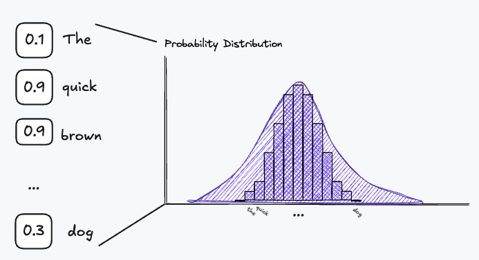
This also means that we want to assign a probability of close to $1$ to the words in the vocabulary which are likely to appear in the context of the target word. This becomes the output of our neural network, meaning we need a neuron to represent each word in our vocabulary, because we need to assign a probability to each one. Now this is not really feasible for large datasets resulting in large vocabularies, which could require hundreds of thousand of neurons. This is also multi-label classification problem, which is in itself a complex optimisation problem, as there are multiple context words that can appear in the context. The innovation presented in the Word2Vec paper decided was to turn this problem on its head. Turning a multi-label classification problem to a binary classification problem. Instead of predicting every word in the context window, we predict whether a single word appears is likely to appear in the context window and which words are not. To be able to do this, we need to construct target word-context pairs. For clarity in the explanations below we show the words themselves and not their index values:

1. Build target word and context pairs 
   using sliding window
   For ex. Target: "quick" | Context: ["The", "brown"]
2. Construct a flattened list of a single target word and single context word pair
   Pairs = [
     ("quick", "The"), 
     ("quick", "brown"), 
     ("brown", "quick"), 
    ...] 

These pairs are our positive samples, now we need to gather negative samples, which are context words which do not appear in the context window for a given word.

3. For each target and context word pair
   3.1 Randomly select words from the vocab that do not fall 
       in context window 
   For ex. quick => ["the", "lazy", "dog"]
   3.2 Construct array of positive context word and negative samples
   For ex. quick => ['fox', "the", "lazy", "dog"]
   3.3 Construct binary label where 1 is the positive context word 
       and 0 for the negative samples
   For ex. [1, 0, 0, 0]

Finally, we can construct a training sample on which we can train our model.

4. Build row in training dataset as (target, context, label)
   For ex. ("quick", ["fox", "the", "lazy", "dog"], [1, 0, 0, 0])

With the new label $\langle 1, 0, 0, 0 \rangle$ we’ve turned this problem into a binary classification problem. Now we only check if the model correctly predicts the positive context word. With the training dataset prepared we can construct the actual architecture for the model:

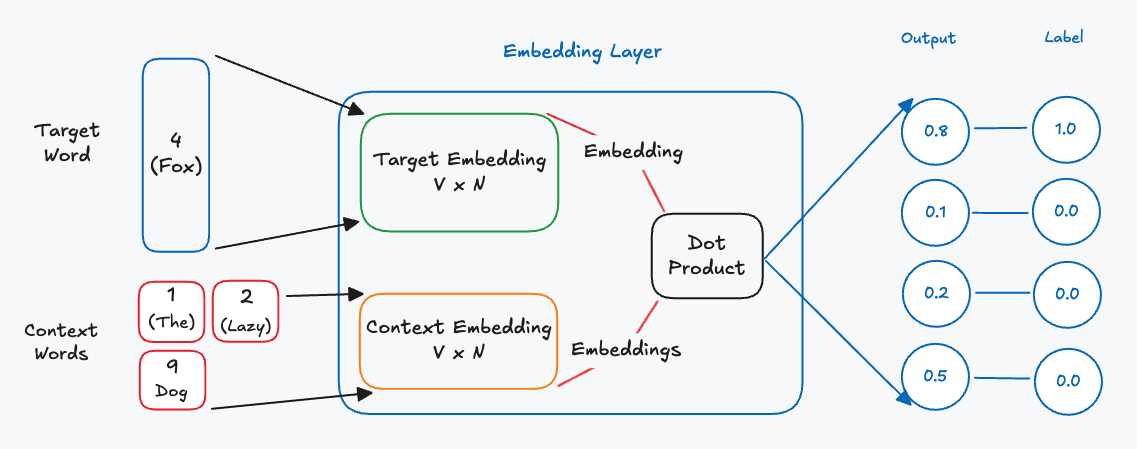
This model is a bit different to a classic neural network, instead of a hidden layer with neurons, we have two embedding layers. Each embedding layer is responsible for resolving the embedding for the target word and context words respectively. The embedding layers themselves are simply matrices representing lookup tables for the word embeddings. Each embedding has rows equal to the size of the vocabulary of the dataset and columns equal to the chosen embedding length. During a forward pass for an input sample we retrieve the target embedding and context embeddings and then calculate the dot product between the two. This is to calculate the similarity of the target embedding with the context embeddings. The result of the dot product is a vector which will then be compared to the label for that specific input sample. The difference between this vector and the label becomes our error, which we can then use to update the embedding matrices. We only update the rows in the embedding matrices for words that were part of the input sample.

Case Studies

Word embeddings are probably the most popular use case for embeddings and this is in part due to LLMs. However, I want to highlight the versality of embeddings, by looking at some case studies of software companies using non-word embeddings.

Case Study: Stitch Fix’s Latent Style

The first implementation we will be looking at is Stitch Fix’s latent style space. Stitch Fix is an online styling service backed by specialised recommendation algorithms powered by … you guessed it embeddings! The full article on their implementation can be found here.

The Problem

Stitch Fix developed a system to recommend clothing items tailored to a user’s style preferences, drawing on their purchase history and past interactions with items. To achieve this, they structured the problem as one of predicting preferences using a method called matrix factorization.

The Solution

The system can be thought of as a large lookup table, or matrix, where the rows represent individual users and the columns represent specific clothing items. Each cell in the matrix contains a value indicating how much a user likes a particular item. The challenge is to predict the values in this table for items a user hasn’t explicitly rated.

The prediction for how much a user $u$ will like an item $i$ is calculated using the formula:

In this equation, $\omega_u$ represents the user’s general tendency to like items (user bias), while $\omega_i$ captures the item’s overall popularity (item bias). The term $v_u \cdot v_i$ measures how compatible the user’s preferences are with the item’s characteristics. This is computed as the dot product of two embedding vectors: $v_u$, which represents the user in a $K$-dimensional feature space, and $v_i$, which represents the item in the same space. By combining these components—user bias, item bias, and the compatibility score—the system can predict how well an item aligns with a user’s preferences. This allows the recommendation engine to suggest items even if the user hasn’t interacted with them directly, resulting in personalized and effective recommendations. The method that they use to find the embeddings is called matrix factorization, we won’t go into how this works, we only care that it can be used to find embeddings. The resulting embeddings are in the form of matrices $U$ and $I$ (not identity matrix), which can be used to calculate the predicted response for an item for a particular user.

The Innovation

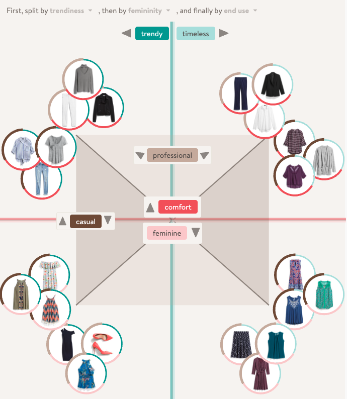
Now what I want to highlight here is not the approach to finding the embeddings, but rather how Stitch Fix interpreted the embeddings and used them to power use cases within their product. The goal was that Stitch Fix wanted to ‘take a step towards understanding style’, so they decided to see what insights they could get from a style latent space. This is the latent space in which the item embeddings live. Recall that the embeddings themselves are multidimensional, and it is not always clear which feature of the data a dimension represents. Stitch Fix attempted to look at which dimensions are the most ‘polarising’. They used a technique called Principal Component Analysis (PCA) which is a dimensionality reduction technique. With this technique they could sort the dimensions by variance, called components for here on, what they realised is that the dimensions themselves could be used as decision trees. Sorting the components by variance allowed them see which components were the most polarising, the first component will represent the most significant division of items. So in terms of style this could represent some broad stylistic preference such as minimalism vs maximalism. They realised that by splitting the data using components they could create meaningful segments of data. This allowed them to reason about the latent space and what they realised was that the latent space seemed to form stylistic client segments:

Case Study: Airbnb’s Listing Embeddings

Airbnb is an online marketplace for short and long term homestays, acting as a broker between rentor and rentee. An interesting feature on their platform is they are able to produce recommendation listings based on similarity. They found that by adding this feature on top of their search functionality they were able to increase their booking conversions.

To be able to serve this feature they needed to create embeddings of their listings. The embedding model is trained on user sessions. A user session can be described as an array of click events, specifically where the user was browsing listings: $\{L_1, L_2, ..., L_B \}$, where $L_i$ is the ID of a listing and $L_B$ is the booked listing. This is to ensure the listings are aligned closer with the listings that are typically booked the most. Airbnb decided to use an approach similar to the Word2Vec approach with negative sampling, with the adjustment that booked listing is also added to each context window as a global context. Recall the Word2Vec model data is trained by attempting to move an embedding towards the postive context example and away from the negative context samples.

The Innovation

Other than the use of the booked the listings as the terminator for the user click sessions, Airbnb also took an interesting approach in dealing with cold-start embeddings. This is the problem of computing an embedding for a completely new listing. The solution Airbnb came up with was to find the three closest listings in terms of listing type, price range, geographic location and calculate the mean between these three vectors. The average then became the new vector embedding.

Multi-Modality

I just also want to add a quick description to give another example of the power of embeddings. Another popular breakthrough that emerged alongside Chat-GPT were DALL-E which is backed by a technique known as diffusion. These models are generative in nature, meaning they generate ‘new’ data based on the user input and its own knowledge. DALL-E takes two types of input, text and sometimes images, the text is typically a description or instruction of what to generate or how to augment the input image. These inputs are then encoded into a latent space which is then given to a decoder model which generates the final image from the values in the latent space. The interesting idea here is that the text and image latent variables share the latent space. To construct this latent space diffusion models typically use a model as CLIP. CLIP is a model, which is used to classify whether a particular caption belongs to an image.

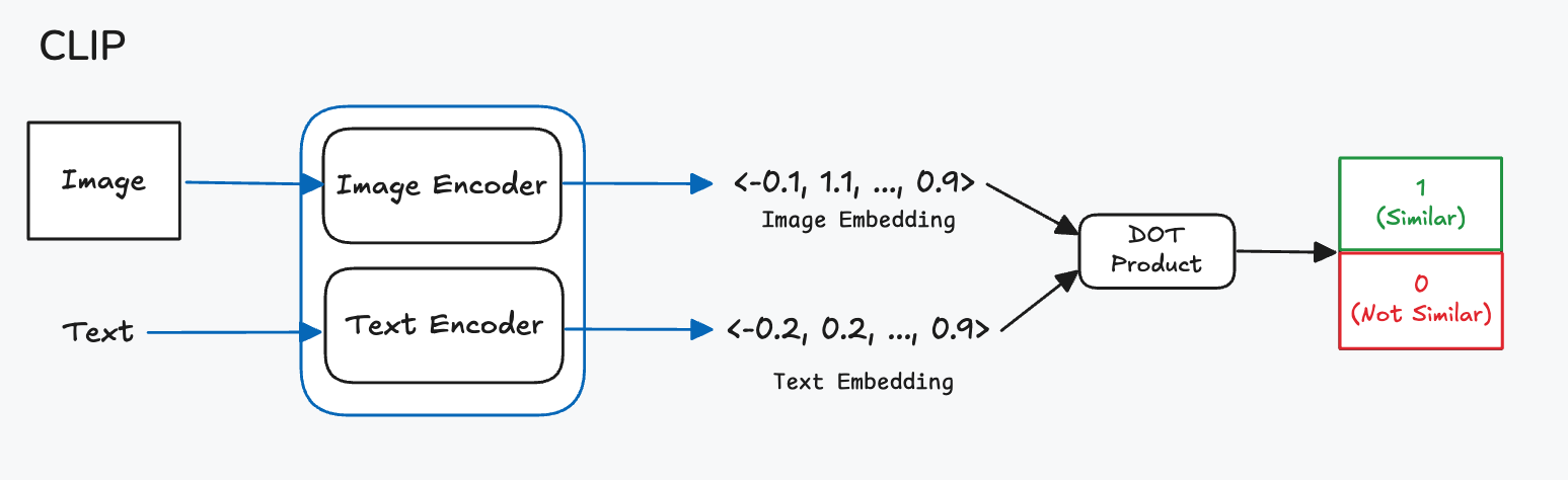
The CLIP model consists of a text and image encoder, here an encoder refers to something that translates some unstructured input to a latent space vector. An encoder is a generalisation of an embedding model. Each encoder is specialised to do this translation for its data type. The exact translation mechanism inside the encoders might be an embedding matrix or a plain neural network, but this is not important for the explanation. To ensure the text and image embeddings are close together in the latent space we train the model such that the dot product between the two embeddings is maximised. This ensures that the embedding vectors will be close together in the embedding space.

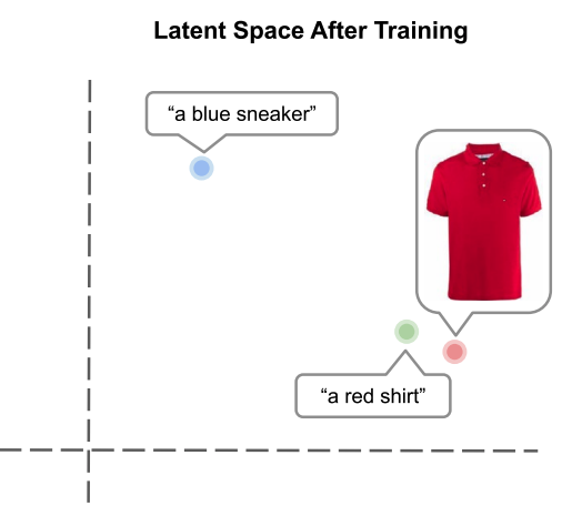
This multi-modality is an incredibly powerful idea, since it allows us to translate objects with completely different underlying structures such that we can reason about them in a shared environment and context.

Conclusion

In this article we looked at the concepts of embeddings in the latent space. We described latent space is the space into which the input is translated, which is presented a different perspective compared to the linear transformation argument from the first article. This also gave us a bit of answer to why neural networks are so good at generalisation and that is they find a better way of representing the data when trained correctly. This is true when looking at word embeddings which are able to encode the syntactic and semantic structures present in the text corpus in a continuous vector space.

Latent spaces were also briefly mentioned to be the ‘environment’ in which a neural network does its reasoning and is also possibly an explanation for why neural networks are able to generalise. This is due to the latent spaces being continuous spaces where the network can interpolate between its knowledge and new unknown data points. Visualised as follows:

Now there is some debate around this statement, so don’t take it as fact, the exact theorems are still being established and might be completely wrong. However, this is still an interesting view of neural networks.

Furthermore, we saw that it is possible to use these embeddings for a variety of downstream tasks such as recommendation or even just to better understand the input data. Embeddings are useful tools for abstraction, they provide a way to abstract the noise from data and also create a space that can support multiple data types. One thing we did not look at is if we can create data using the properties of the latent space instead of just querying it. This is also a very exciting research area, but requires us to use a specialised neural network that attempts to model this latent space, by training it to rebuild the input from the latent space. This is where auto-encoders come into play, but that will be a story for another day.

Code

• Word2Vec Model I wrote for experimentation

Further Reading

• Graph Embeddings
• Hierarchial Embedding Theory - Math heavy, but cool idea
• Representational Learning Survey - Long, but informative

References

• Word2Vec Paper
• Representations in Deep Learning and NLP - Great Read
• Latent Style
• Airbnb Listing Embeddings